"Determining Tire characteristics through data driven modeling"

This was our so-called Bachelor End Project or BEP.  Our group consisted of

• E. Figueiras
• M. Kleijwegt
• N. Romer
• A. Soerdjbalie

We tried to investigate the characteristics of the tires of model RC cars. By developing a new method for finding the characteristics at model scale, a cheap and repeatable method for finding the grip coefficients can be realized.

My work mainly focused on the experimental setup, specifically writing the software to drive the car and gather data at the same time.

We used GitHub to collaborate on all of our code, including the paper. We stored it under the organization https://github.com/BEPAutonomousDriftingCar. However, we transferred the organization to the next group after finishing the project. So not all code will be ours. The main repositories are

• Donutdevice - our C++ ROS package running on the pi gathering data
• AutonomousDriftingCar -  our C++ teensy code for reading the sensors
• Matlab
• Paper

Experimental setup

In order to determine the tire characteristics of the scaled vehicle, a good testbed is necessary. We concluded from a model that the following variables are required to measure the tire characteristics:

• the linear accelerations of the car
• the linear and angular velocities of the car
• the steering angle of the front wheels
• the angular velocities of the wheels

The experimental setup consists of a modified scaled RC car with an onboard IMU, feedback servo, and a tachometer on each wheel. Moreover, a motion capture system, or MoCap, was used to provide millimeter precision localization. The IMU is used to measure the velocities and accelerations of the car. The feedback from the servo is used to determine the steering angle. The tachometers are used to measure the angular velocity of the wheels. The MoCap was used to check and calibrate the signal coming from the IMU. However, the noise on the MoCap location signal, which is amplified by differentiation, made it unfit for this research.

Car

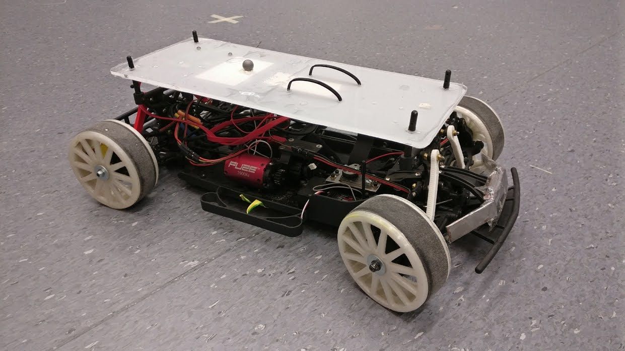
The RC car is a Losi TEN Rally-X. It is a 1:10 scale car with 4WD powered by a 2s 6000 mAh LiPo battery and a 3900KV Fuze Brushless DC motor. With this battery, the car is able to drive at speeds between 1.5 and 15 m/s. To meet the assumptions of the Bicycle model, the suspension of the car was replaced with stiff turnbuckle rods to eliminate the degrees of freedom of roll and pitch. The wheels are custom 3D-printed rims with grip tape applied to simulate tires and fitted with 2 magnets each. When the magnets pass a hall-effect sensor on the car a signal is created of 2 pulses per revolution. The hall-effect sensors and the magnets make up the tachometers of the car. Another set of wheels with space for 24 magnets was created, but due to a lack of time, no tests were conducted with these. The IMU was mounted in the center of gravity of the car, preventing angular velocities from influencing the accelerometer. Finally, the standard servomotor was replaced by a robot servo motor, which allowed for reading the angle from the servomotor angle sensor.

MoCap

The MoCap is used as a positioning system. A MoCap system cannot be regarded as an onboard sensor, as it requires an area with aligned cameras. However, in this case, it is used as a replacement for a GPS sensor. The MoCap system enables us to do testing inside, something which is not possible with a GPS system. Finally, the MoCap system was ready to use and already connected with ROS, using a sampling rate of 120 Hz.

Data acquisition and processing

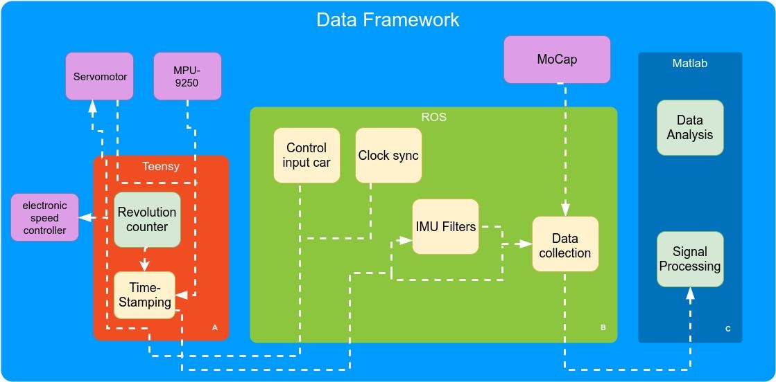
Data acquisition was done using a ROS (Robot Operating System) based system. The sensors were connected to a Teensy 3.6 prototyping board running a custom ROSserial node, connected to a Raspberry Pi 3 model B running ROS. The custom ROSserial node uses an interrupt-controlled program to gather sensor data in a fast and accurate way. Moreover, onboard hardware timers were employed as pulse counters for the tachometer signal. The MoCap is connected to the system utilizing the lab's Wi-Fi network.

Further communication was done using a self-written ROS package. After data collection, further processing was done using Matlab. The figure further elaborates on the data acquisition framework.

ROS

Implementing ROS on the testbed provided it with some key components needed for accurate testing. Since ROS has already been established as a research and prototyping framework, a lot of packages are already developed for this operating system and are easily available. One key component is timestamping. To provide usable data, the testbed needs a timestamping method. ROS automatically syncs all the clocks on every device providing a convenient solution to this problem. Furthermore, our testbed contains a simple IMU which does not provide all data that a more advanced IMU might offer, like orientation or sensor fusion between the magnetometer and gyroscope signal. There- fore a complementary filter was used in ROS to generate this data.  The complementary filter was chosen for this purpose as its transfer function and the implementation is the same as a Kalman filter. However, the complementary filter has improved response time. Moreover, the MoCap generated its data already in ROS, which meant combining everything in ROS would be a simplification. Also, ROS offers convenient data recording options called ROSbags, which can be imported into MATLAB for further analysis.

Sampling

The sampling rate for our experiments was set at 120 Hz. The MoCap already operated at this sampling rate and to simplify synchronizing our data points one sampling rate was used. Moreover, if all sensors would work on the same sampling rate, this would reduce the hardware requirements on the Teensy and reduce the need for data interpolating. Since a lot of noise was apparent on the IMU signal in initial tests, the decision was made to employ the built-in Digital Low Pass Filter (DLPF) on the IMU, to decrease noise and data rate at the same time. However, this would create a delay in our signal. To prevent this delay from becoming significant, a limit of 10ms signal delay was chosen. A 92 Hz DLPF was chosen since it only created a delay of 7.8 ms, but would decrease the data rate significantly without losing data points. To prevent signal aliasing, a sampling rate of 92 Hz or higher is required. Our sampling rate of 120 Hz fills this requirement

Experiments

The experiments can be classified into three groups. The first set of experiments is carried out in a straight line (longitudinal motion). During these experiments, the car accelerated and braked while driving straight ahead. The second set consists of steady-state cornering experiments (lateral motion). Steady-state cornering means cornering at a constant longitudinal velocity and constant steering angle. Finally, the third set of experiments takes both lateral and longitudinal motion into account. Variables of the tests are acceleration/deceleration for longitudinal motion, longitudinal velocity, and steering angle for lateral motion, and these three combined for combined motion. The variables were slightly increased in each experiment in order to determine the transition from linear to nonlinear behavior.